#01 broccoli → lobster
wrong class · same style
Poster notes: abstraction retrieval on Toronto Scenes, and content/style probing on Things × ArtBench. Figures, failure cases, and extra plots are below.
Two measurements on frozen ViT-B models: (1) how retrieval changes when Toronto Scenes photographs are driven toward line drawings, and (2) whether a linear probe on CLS can recover artistic style when raw cosine kNN cannot.
Source photographs come from the Toronto Scenes dataset. We morph
each scene with SDXL + ControlNet along an abstraction axis
λ ∈ [0,1] (line drawing → photograph). Models are evaluated with
zero-shot instance / category retrieval along the spectrum.
Expanded figures and curves live on the
visual abstraction report.
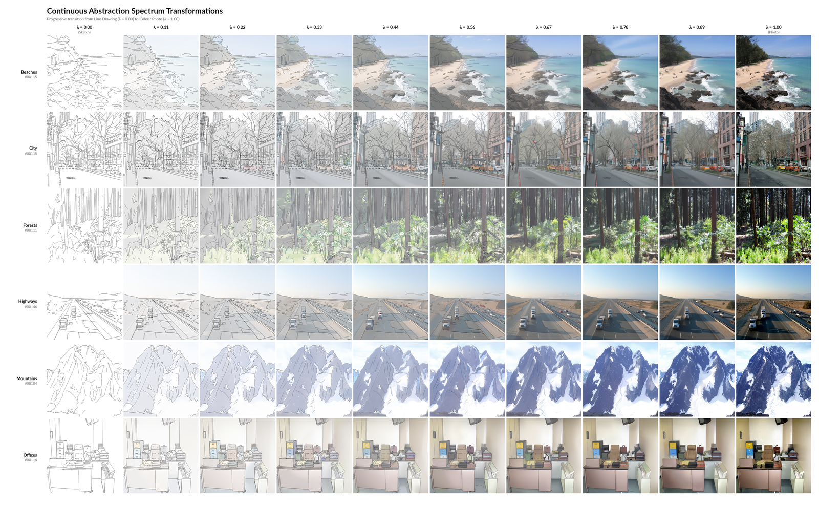
How the spectrum is built (edge map source, the blend and ControlNet schedule behind λ, the fixed 0.35 strength, LPIPS/SSIM validation) is written up under generation pipeline.
UCAST-style pairings[1] give independent content and style labels using THINGS objects[2] and ArtBench styles[3]: the same object under many artistic styles, and the same style across many objects. This enables dual zero-shot retrieval (content vs style). See the zero-shot style report for the full probing suite.
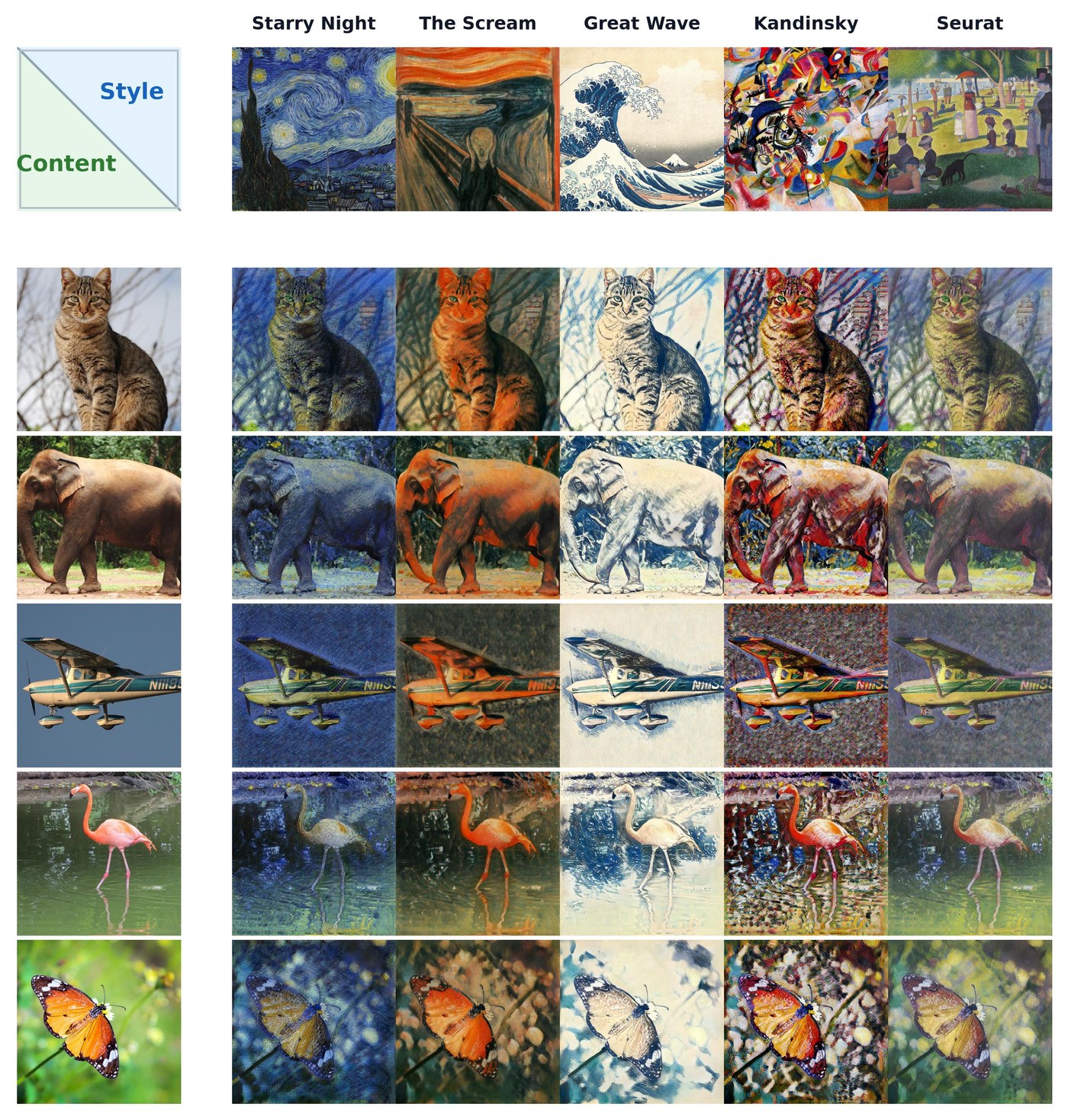
The 5×5 here is a display subset; the probes use 1,000 ArtBench styles. Content and style pools, the AdaIN forward pass, and the split rule are under UCAST pipeline.
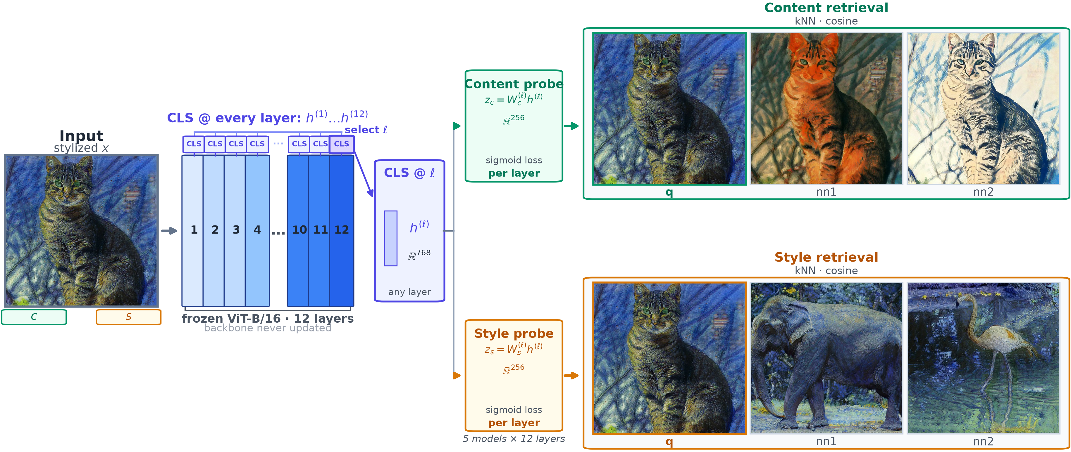
Freeze a ViT-B/16 backbone. At every layer ℓ ∈ {1…12}, take the
L2-normalized CLS token h^(ℓ) ∈ R^768 and train two independent
Linear(768, 256) heads, one for object identity and one for
artistic style, with a pairwise sigmoid focal loss over the
512 × 512 cosine matrix of a class-balanced batch. Evaluation is
zero-shot kNN with cosine similarity (Recall@1 / mAP); the learned temperature
and logit bias are training-only.
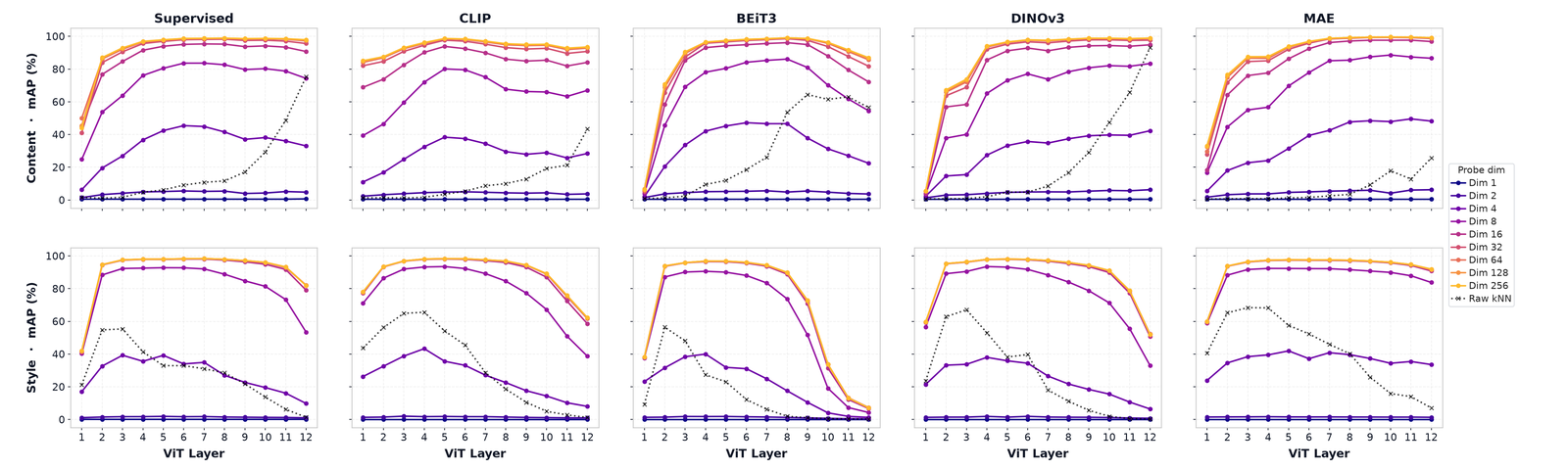
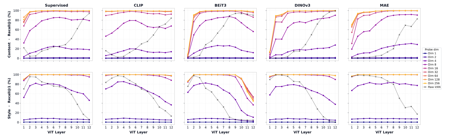
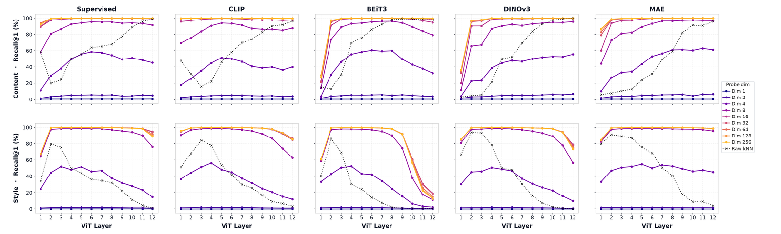
Across Supervised, CLIP, BEiT3, DINOv3, and MAE, raw late-layer CLS style retrieval is under 1%. Trained probes raise style Recall@1 / mAP; higher probe dimensions help, and the unprobed CLS baseline stays low in late layers.
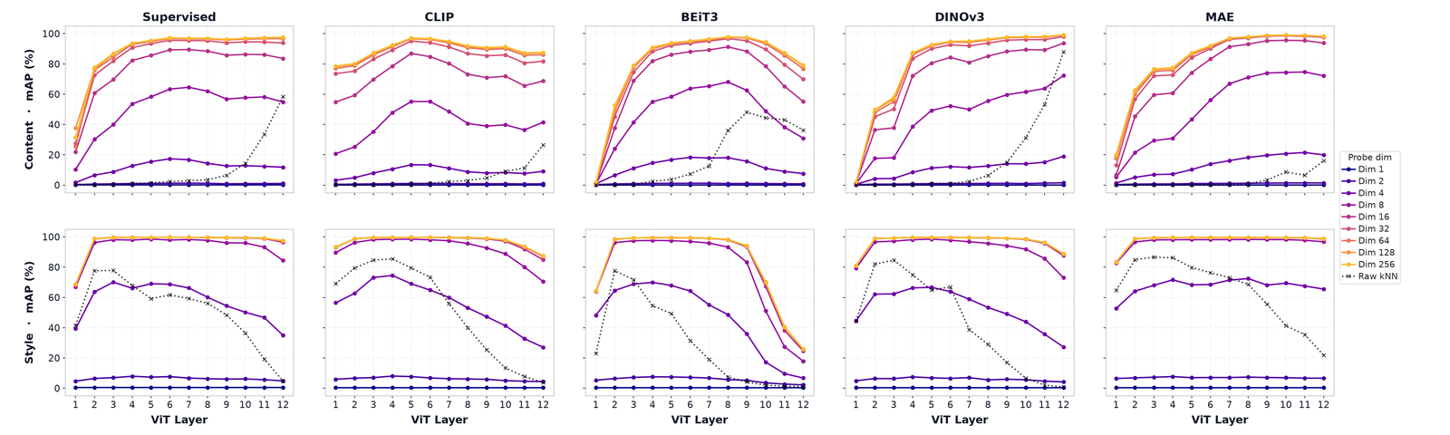
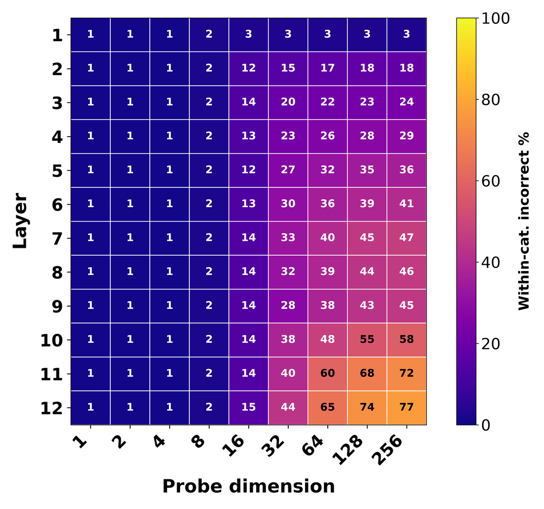
The poster keeps this single style heatmap for simplicity. Full content+style grids, per-split breakdowns, Recall@1 curves, and the Matrioshka re-normalization study are in Bonus analyses.
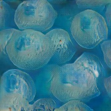
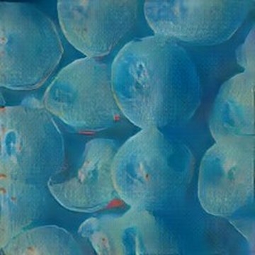
The poster shows four representative pairs. Below are curated incorrect neighbors from the DINOv3 dim-256 content probe. Several pairs share artistic style and differ in object class (tagged below).
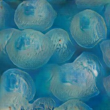
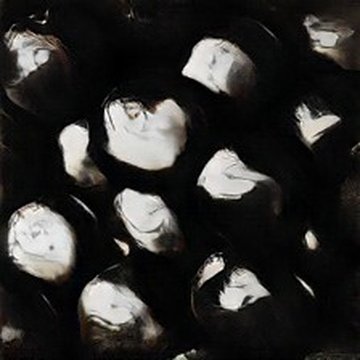
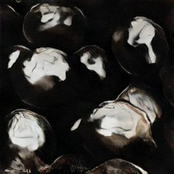
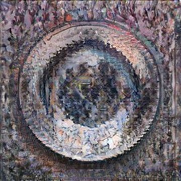
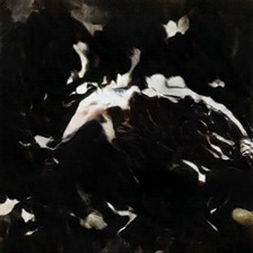
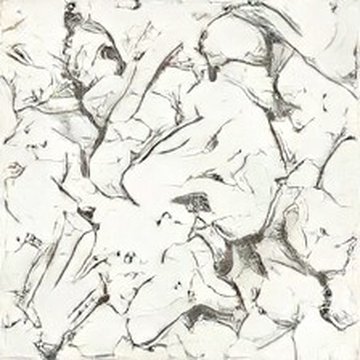
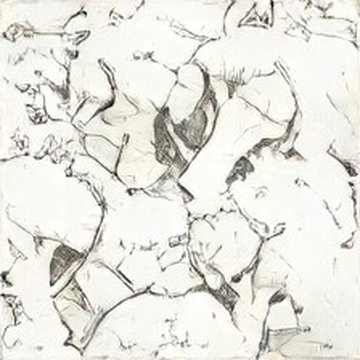
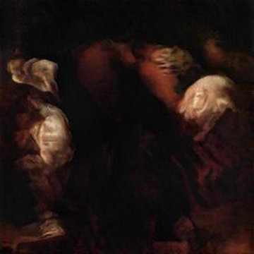
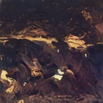
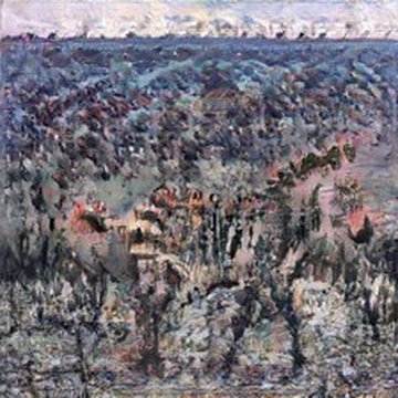
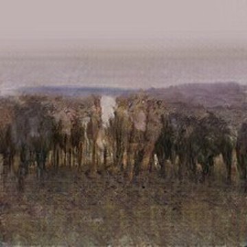
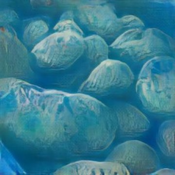

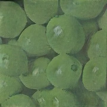
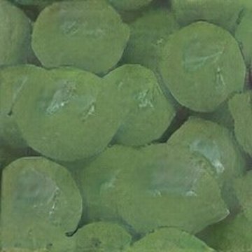

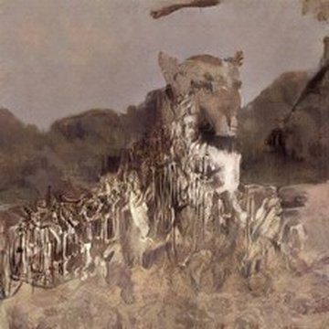
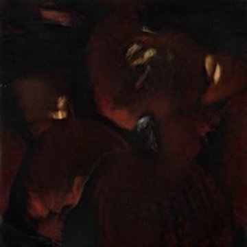
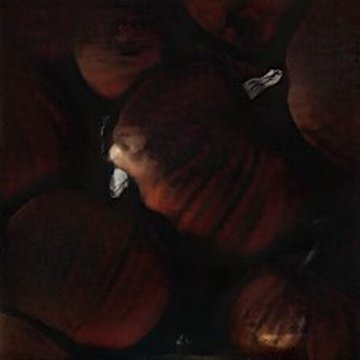
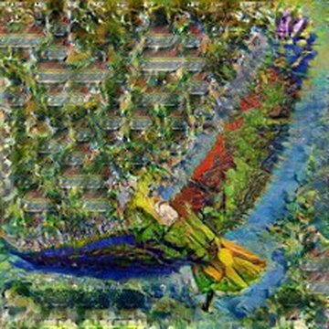
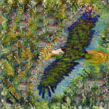
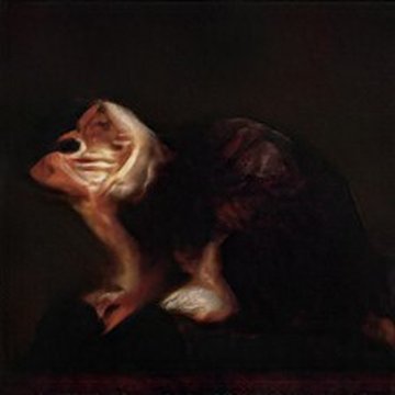



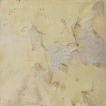
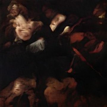
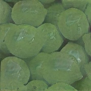
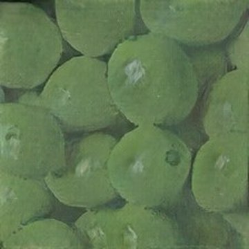


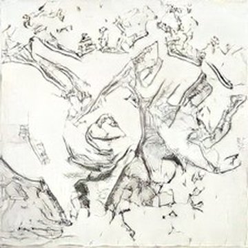
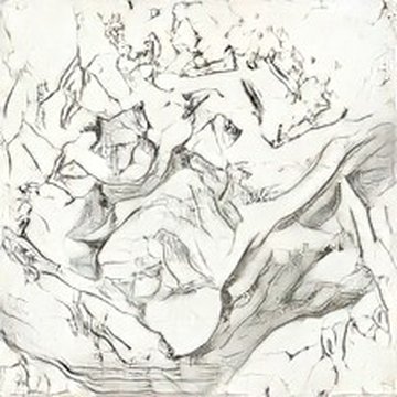
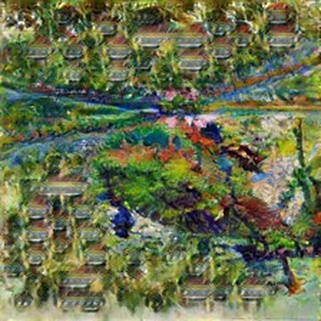
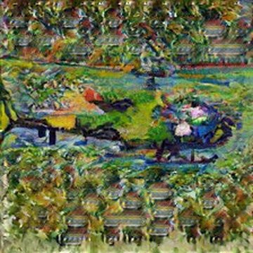
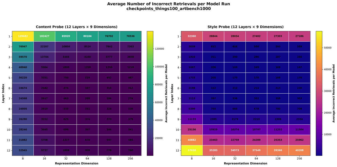
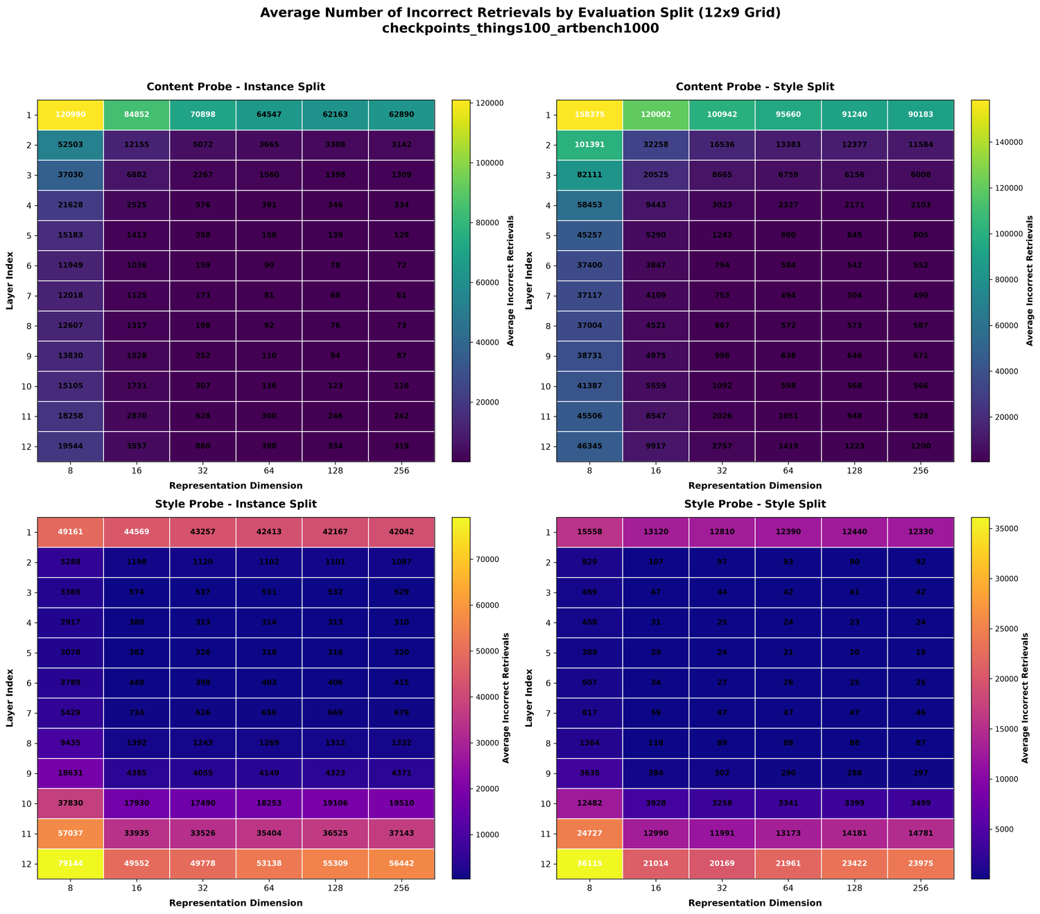
Plots that did not fit on the poster: retrieval grids, within-category heatmaps, total-error heatmaps, and nested-dimension (Matrioshka) re-normalization.
Style and instance splits for both mAP and Recall@1. Solid curves = probed dimensions; dashed = raw CLS kNN baseline.
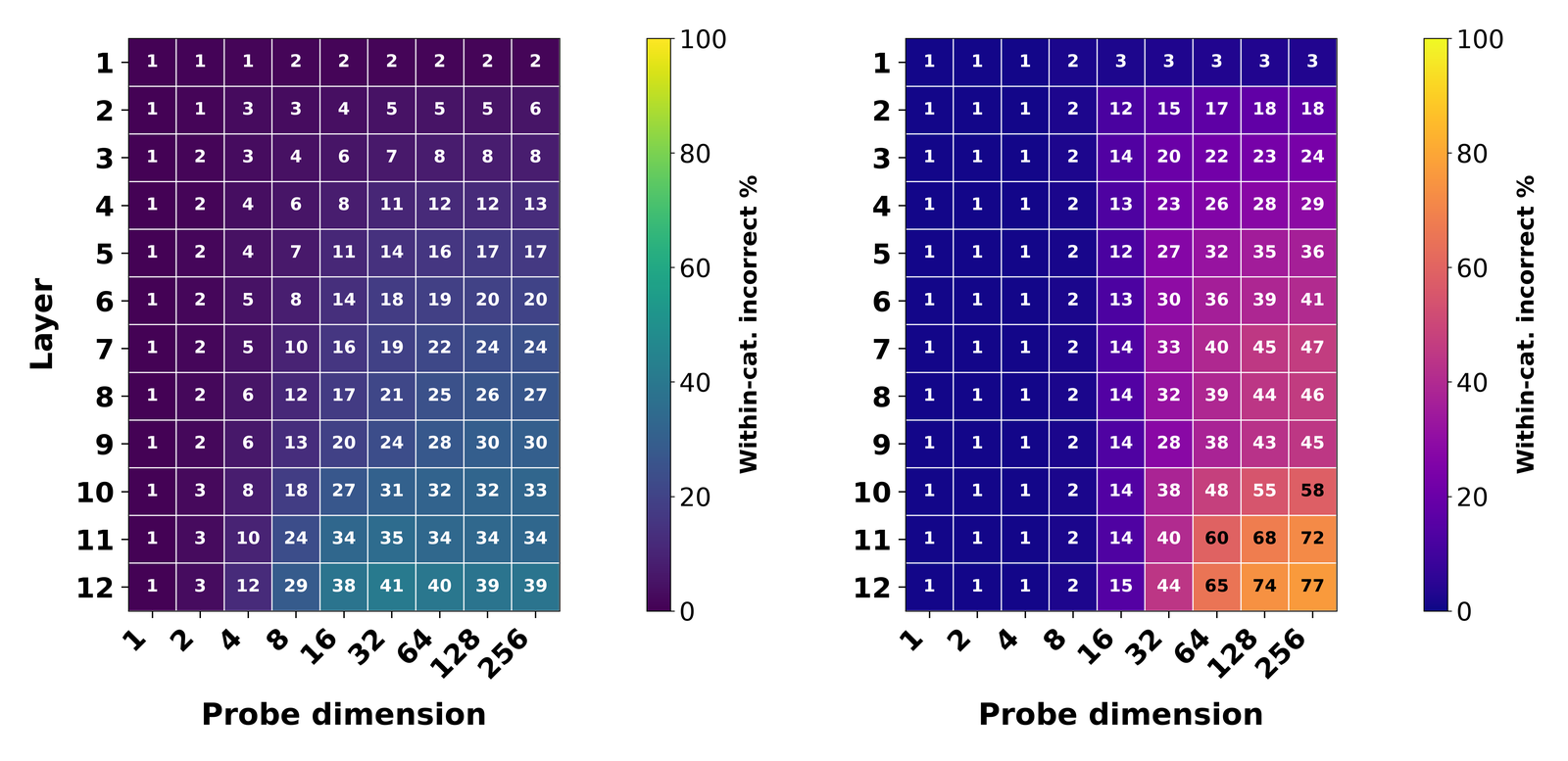
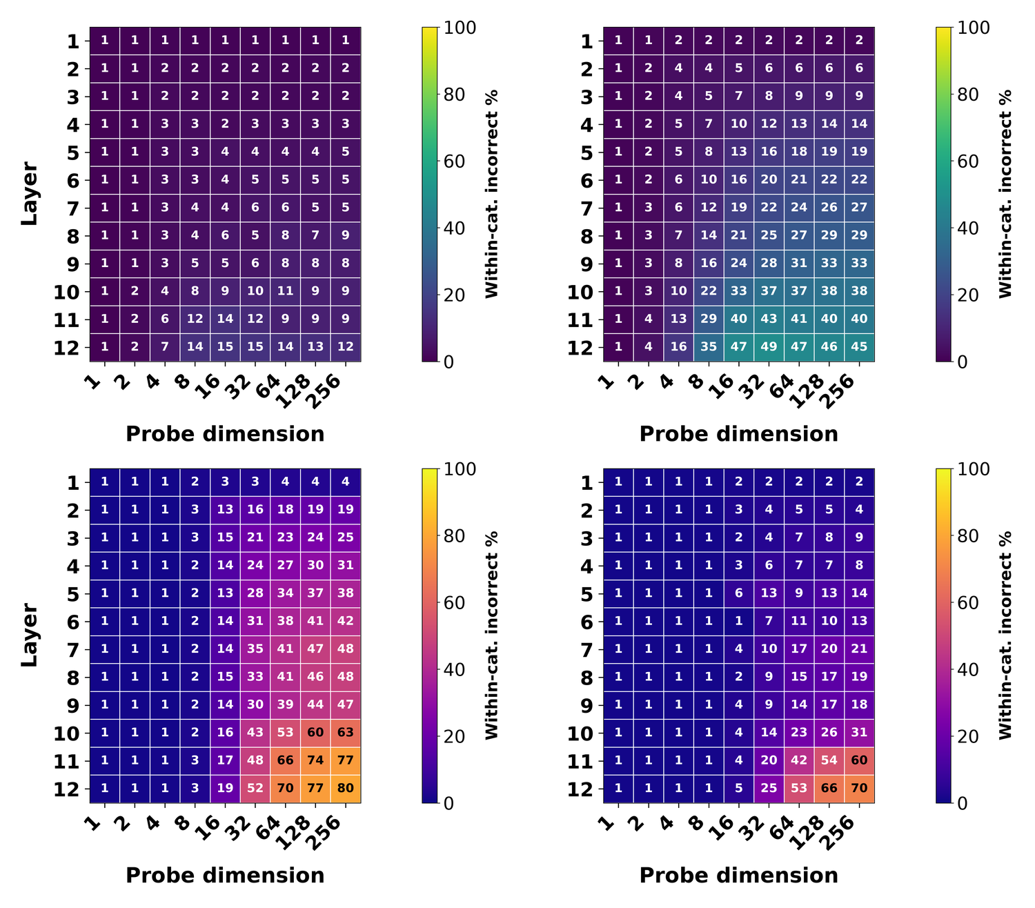
Fraction of incorrect retrievals that still land in the same content category. Useful for separating style-looking mistakes from random neighbors.
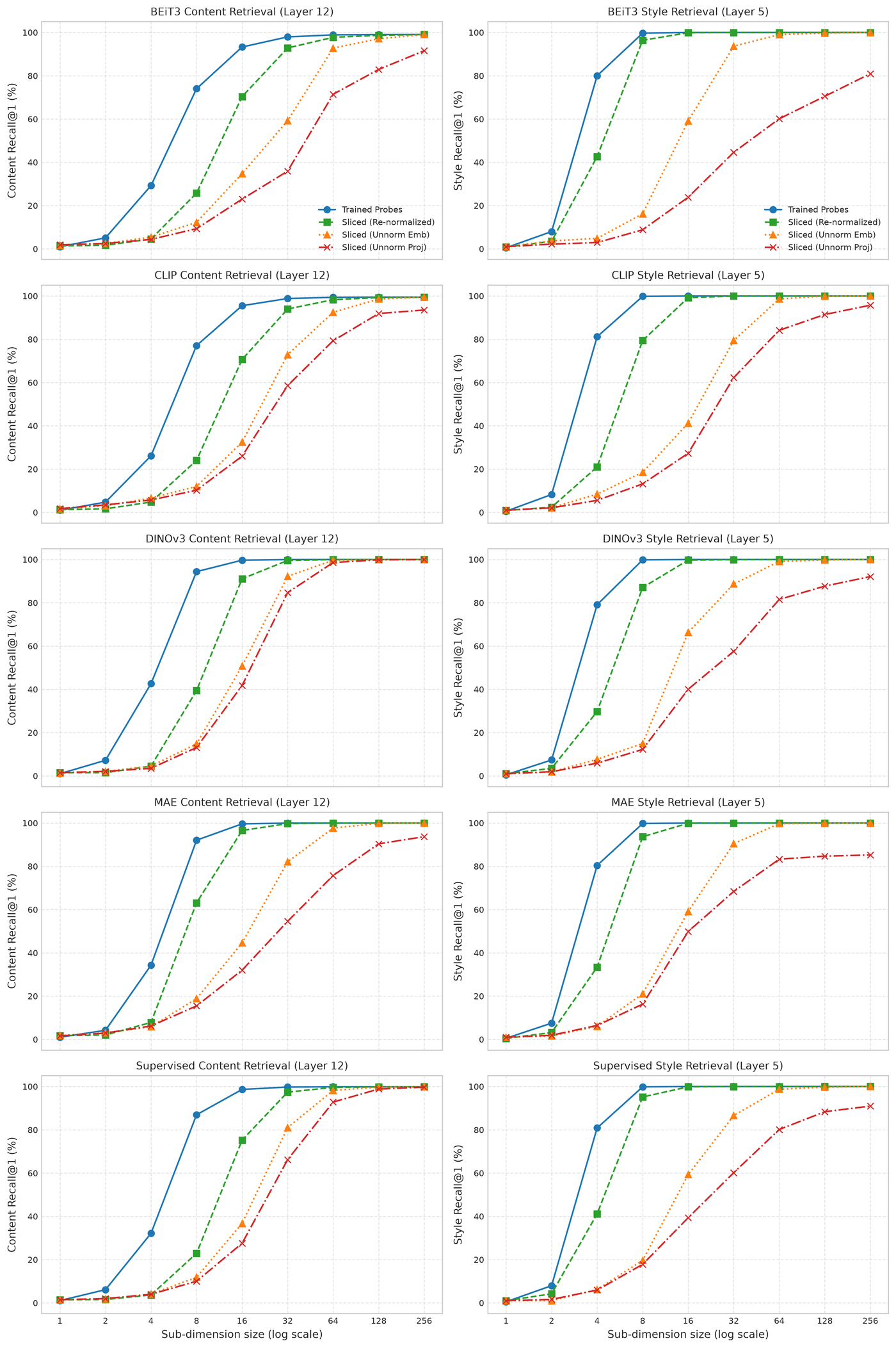
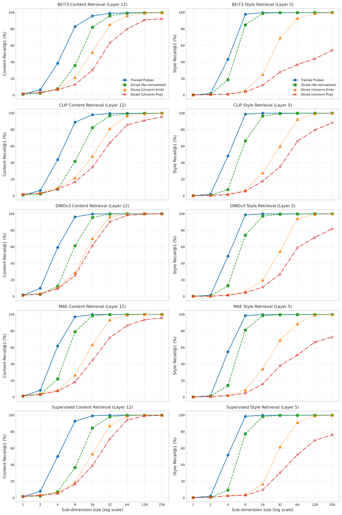
Nested slices of the 256-D probe test whether early dimensions already carry the
task, and whether L2 re-normalization of a truncated prefix matches the full vector.
For style, small K with re-norm stays close to the full 256-D probe.
Without re-norm, truncated prefixes degrade.
The probe head is Linear(768, 256, bias=False) followed by L2
normalization, so the 256-D output lives on the unit sphere and
z @ z.T is already a matrix of cosine similarities. Training turns
that matrix into logits with a learnable scale and shift,
logits = (z zᵀ) · exp(t′) + b, and compares it against a binary
target: 1 where two images share a label, 0 otherwise,
diagonal dropped so self-pairs never contribute.
Every off-diagonal entry is then its own binary decision. With
p = σ(logit), a true positive pair contributes
(1-p)^γ · log p and a true negative contributes
p^γ · log(1-p), both computed through F.logsigmoid so
large-magnitude logits do not underflow. The γ factor is the focal
term from Lin et al.[4]: pairs the probe already scores
correctly get discounted, and the gradient concentrates on positives that are
still far apart and negatives that are still too close. We use
γ = 1.0.
Detection focal loss puts α = 0.25 on the foreground class because
foreground boxes are the rare ones. In an N×N pair matrix the rare class is the
positive, so α is flipped to 0.75 and sits on the
positives. At C = 32 classes and M = 16 images per
class, each row has 15 positives against 496 negatives, roughly 33:1.
That 33:1 is handled before α ever applies. Positive and negative
losses are summed and divided by their own counts (sum / n_pos,
sum / n_neg), which removes the raw count imbalance on its own;
α = 0.75 against 1 - α = 0.25 then leaves a mild 3:1
tilt toward pulling positives together. Final loss is
pos_loss + neg_loss.
The sampler draws C = 32 classes and M = 16 images per
class without replacement, giving N = 512, then shuffles the indices
so the target is not block-diagonal in memory layout. The content sampler groups
by instance/object label and the style sampler groups by style label, so the two
probes see different batch compositions at the same layer. The style split
sometimes has fewer than C usable classes, in which case
C is clamped to what exists.
There is an InfoNCE version of the training script and it works, but the softmax couples every pair in a row: raising one similarity lowers the others whether or not they are wrong. Sigmoid scoring treats each pair independently, which is closer to what evaluation asks (is this neighbor the same class, yes or no) and is the same shape as SigLIP-style pairwise sigmoid objectives, minus the text tower. Square sampling then fixes the positive count per batch, so the N×N target is never almost entirely zeros.
γ=1.0, α=0.75, τ=0.0667 (init scale ≈ 15), b = -10.0.1e-3, cosine annealing.1e-2 on proj.weight only, not on t′ or b.
Both t′ and b are trained, and neither survives into
evaluation. Retrieval is plain cosine kNN on the normalized 256-D embeddings,
scored with Recall@1 and mAP, so whatever calibration the scale and bias learned
is irrelevant at test time.