Visual abstraction and neural representations
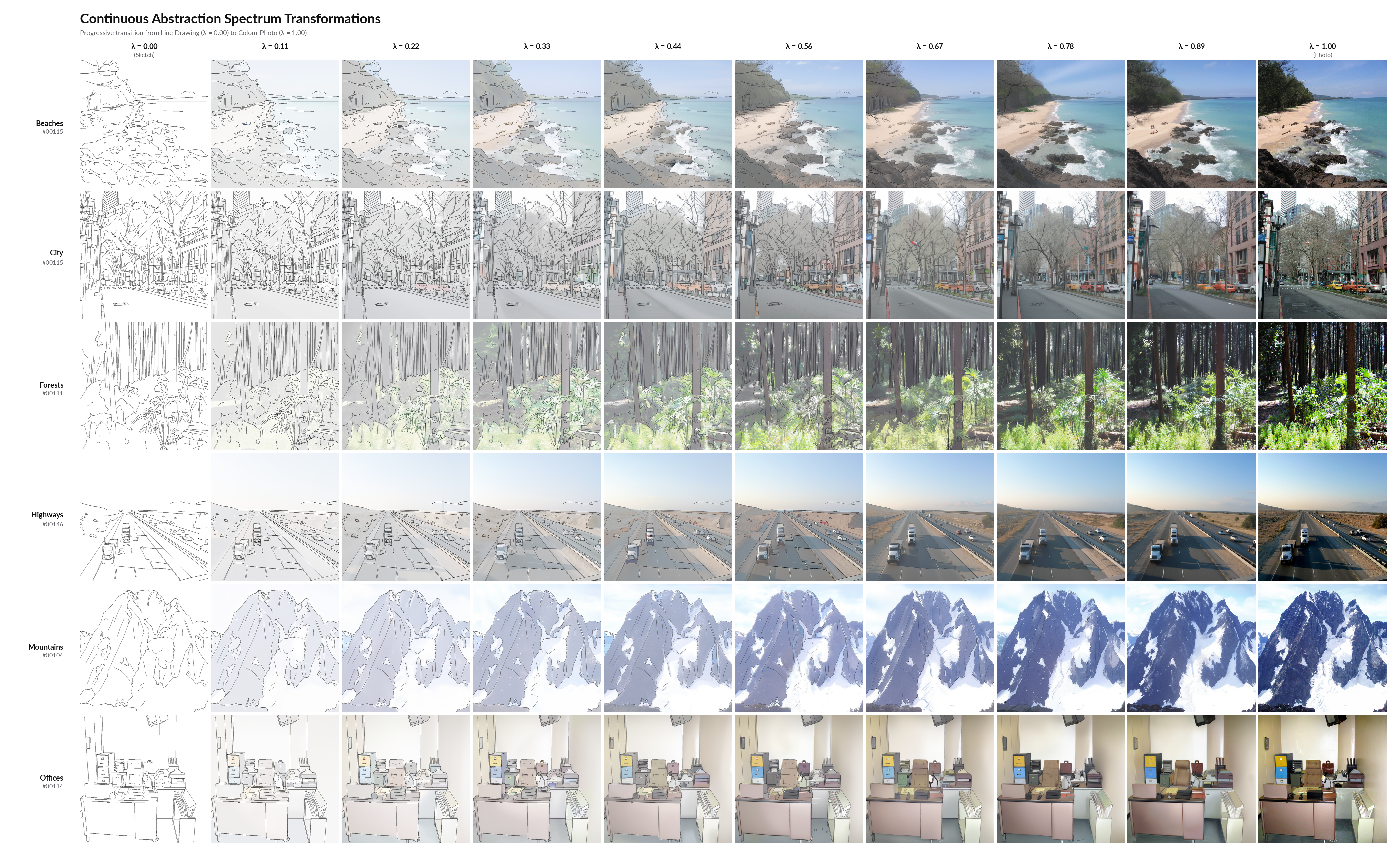
Diffusion Abstraction Spectrum (DAS) on Toronto Scenes: the same photographs morphed from line drawings (λ=0) to photos (λ=1), scored with frozen ViT-B retrieval.
Overview
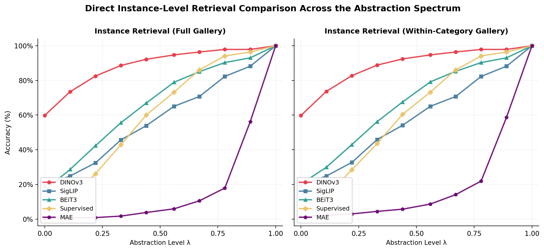
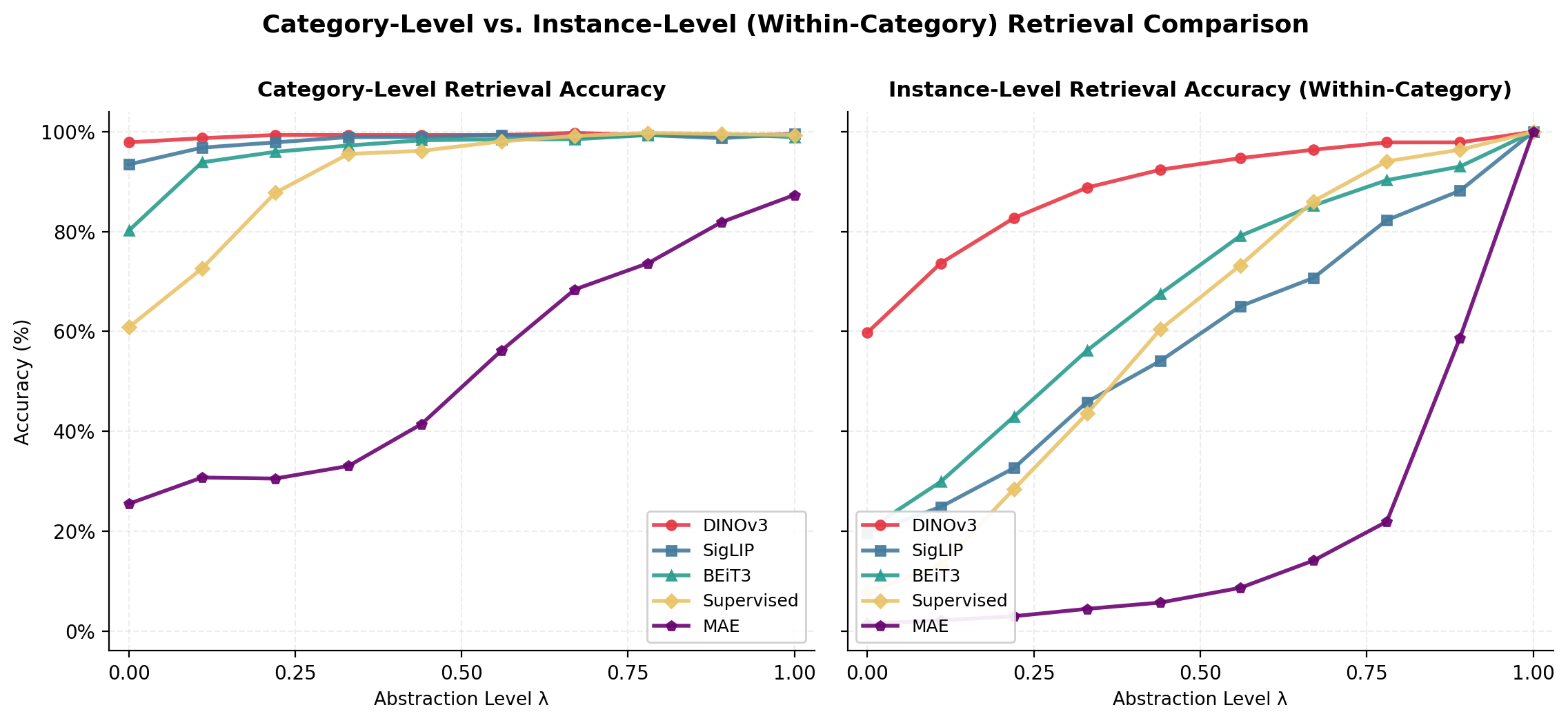
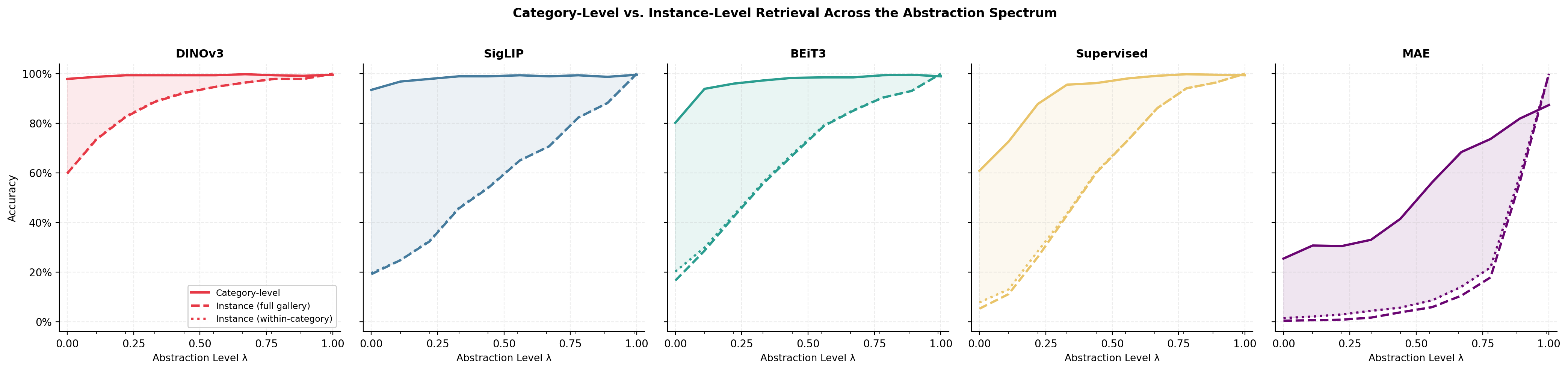
We take photographs from the Toronto Scenes dataset and morph them toward sketches. Retrieval at the sketch pole is not the same across ViT-B checkpoints: DINOv3 stays high on category R@1; MAE does not.
Diffusion Abstraction Spectrum
Source images are from Toronto Scenes. We morph each scene with
SDXL + ControlNet along λ ∈ [0, 1] (line drawing → photograph).
The probe set used here is 475 scenes × 10 levels (4,750 images). Models are scored
with zero-shot category and instance retrieval along the spectrum.

Generation pipeline
Every one of the 475 scenes goes through spectrum_pipeline.py once and
comes out as 10 images, so 4,750 total. Levels are
λ = i / (n_levels - 1) with n_levels = 10: 0.00, 0.11,
0.22, and so on up to 1.00. Seed is fixed at 42 for the whole run. The strip and
grid above are outputs of this script.
Inputs per scene
- Photograph loaded as RGB and resized to
1024×1024. -
Edge map: if a companion
{stem}_LD.pngexists it is used and inverted, giving white lines on black, which is what ControlNet scribble expects. Otherwise we run HED (lllyasviel/Annotators). Canny is a flag in the code; HED is the default used for the paper numbers. The edge map is resized to1024×1024as well. -
Prompt: if the caller does not pass one, BLIP
(
Salesforce/blip-image-captioning-base) captions the photograph. BLIP is unloaded before SDXL is built, otherwise both do not fit in VRAM.
Models
SDXL base (stabilityai/stable-diffusion-xl-base-1.0) with
xinsir/controlnet-scribble-sdxl-1.0, Euler ancestral scheduler, fp16,
VAE slicing and tiling on, model CPU offload on CUDA. One pipeline is loaded and
reused across all scenes in a batch.
What λ actually controls
Two knobs move together. The img2img init image is a straight pixel blend,
start_image = Image.blend(edge_rgb, natural, alpha=λ), so λ=0 starts
from pure edges and λ near 1 starts from something very close to the photograph.
The ControlNet conditioning scale is
ccs = 0.9 - (λ * 0.85), which runs from 0.9 at λ=0 down to 0.05 at
λ=1: the line drawing is enforced hard at the abstract end and barely at all at the
natural end.
Denoising strength is fixed at 0.35 at every level, with
guidance_scale = 7.5 and num_inference_steps = 50. That
is deliberate. The abstraction level comes from the blend and the ControlNet scale,
and diffusion is only there to make the blend look like a coherent image rather
than a photograph with lines drawn on it. At λ ≥ 0.99 generation is
skipped entirely and the original photograph is copied, so the λ=1 end of the
spectrum is real data, not a reconstruction.
| λ | blend alpha | ControlNet scale | strength |
|---|---|---|---|
| 0.00 | 0.00 (pure edges) | 0.90 | 0.35 |
| 0.33 | 0.33 | 0.62 | 0.35 |
| 0.67 | 0.67 | 0.33 | 0.35 |
| 1.00 | copy original | n/a | n/a |
Outputs and validation
Each scene gets its own directory holding lambda_{lam:.2f}.png for the
ten levels, plus edges.png, caption.txt, and
validation.json. Validation scores every level against the natural
photograph with LPIPS (alex) and SSIM at 512, then checks that LPIPS
is monotonic walking from λ=1 back to λ=0. A scene that fails that check usually
means the edge map was bad, and it is worth opening by hand before the scene enters
the retrieval set.
The 475 source photographs used for retrieval are the Toronto Scenes images on this
page; the pipeline README licenses the DAS release as Places365-derived. A second
script, cp_ld_pipeline.py, runs the same construction for paired CP/LD
stems with BLIP-2 captions, and is not used for any number reported here.
Retrieval across λ
| Model | Pretraining | Category R@1 (λ=0) | Instance R@1 (λ=0) |
|---|---|---|---|
| DINOv3 | Dense SSL | 97.9% | 59.8% |
| SigLIP | Vision–language | 93.5% | — |
| BEiT3 | Masked multimodal | 80.2% | — |
| Supervised | IN-21k | 60.8% | — |
| MAE | Generative SSL | 25.5% | 0.4% |
Geometry note
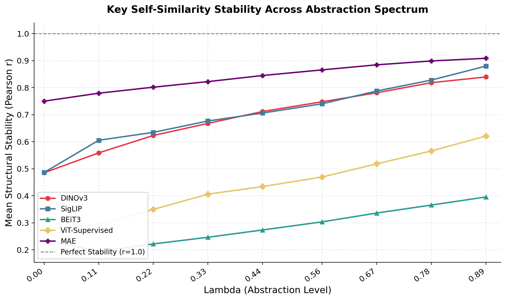
MAE can keep relatively high attention-key self-similarity across λ while category/instance retrieval at λ=0 is still low. Layout stability on this metric does not by itself explain the retrieval numbers.